VGGNet and Tiny ImageNet
In this post, I describe the results of implementing and training a variation of the VGG-16 convolutional neural network (convnet). The convnet is trained and evaluated on the Tiny ImageNet dataset. Tiny ImageNet spans 200 image classes with 500 training examples per class. The post also explores alternatives to the cross-entropy loss function. And, finally, I show pictures with their predictions vs. true labels, saliency maps, and visualizations the convolution filters.
Introduction
ImageNet, and Alex Krizhevsky’s “AlexNet”, sparked a revolution in machine learning. AlexNet marked the end of an era of hand-crafted features for visual recognition problems. In the few years that followed AlexNet, “deep learning” found great success in natural language processing, speech recognition, and reinforcement learning. Again, machine-learned features supplanted decades worth of hand-crafted features.
With only 2 hours of GPU training time, costing about $0.50 using an Amazon EC2 spot instance, it was not difficult to reach 55% top-1 accuracy and nearly 80% top-5 accuracy. At this level, I was often misclassifying many of the same images that the model predicted incorrectly.
Objectives
- Design and train a high-performance deep convnet
- Implement saliency: Where in the image is the model focused?
- Visualize convolution filters
- Experiment with alternative loss functions:
a. Smoothed cross-entropy loss
b. SVM
All code is available in this github repository. Also, the notebooks can be found on Gist:
Dataset
Stanford prepared the Tiny ImageNet dataset for their CS231n course. The dataset spans 200 image classes with 500 training examples per class. The dataset also has 50 validation and 50 test examples per class.
The images are down-sampled to 64x64 pixels vs. 256x256 for full ImageNet. The full ImageNet dataset has 1000 classes vs. 200 classes in Tiny ImageNet.
Tiny ImageNet is large enough to be a challenging and realistic problem, but not so large as to require days of training to see meaningful results.
The Model
This paper by Karen Simonyan and Andrew Zisserman introduced the VGG-16 architecture. The authors reached state-of-the-art performance using only a deep stack of 3x3xC filters and max-pooling layers. I used VGG-16 as a starting point because I found the elegance and simplicity of this model appealing. The VGG-16 architecture is also a proven performer.
Because Tiny ImageNet has much lower resolution than the original ImageNet data, I removed the last max-pool layer and the last three convolution layers. With a little tuning, this model reaches 56% top-1 accuracy and 79% top-5 accuracy.
I didn’t use pre-trained VGG-16 layers from the full ImageNet dataset. I trained from scratch using only the Tiny ImageNet training examples.
Training
Settings
Here is a summary of the training settings:
- learning rate = 0.01
- Decay by 5x when validation accuracy stops improving
- 3 learning rate decays before training is terminated
- L2 regularization on all layers (single regularization coefficient)
- 50% dropout on fully-connected layers
- He initialization on all weight matrices:
- Optimizer: SGD with Nesterov Momentum (momentum = 0.9)
- batch-size = 64
A few key points:
- I’ve found SGD with Nesterov momentum works as well as, or better than ADAM or RMSprop. The hyper-parameters for SGD are less finicky to set, and it seems to learn as quickly as ADAM.
- For ReLU layers, He initialization works excellently. The network implemented here has 13 layers of weight matrices. With He initialization, my activations were well-bounded right to the last layer. This initialization eliminated the need for batch normalization.
- Learning rate decay is almost universally applied in published papers, and for a good reason. The plot below illustrates the significant accuracy improvement after the first learning rate decay. With a high learning rate, you start to overfit your mini-batches as you get close to a good local minimum. By decaying the learning rate, each mini-batch makes a smaller “vote” on which way to move.
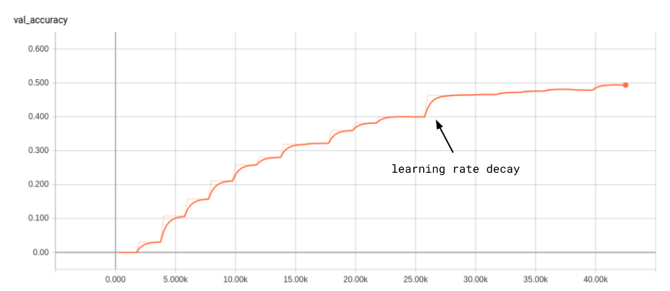
Figure 1. Accuracy vs. training batch. 1.5k batches per epochs: 27 epochs total.
Loss Function
I experimented with three different loss functions:
- Cross-entropy loss
- Smoothed cross-entropy (small probability added to incorrect classes)
- Support Vector Machine
For smoothed cross-entropy, I assigned a probability of 0.9 to the correct class and divided the remaining 0.1 probability mass among all 200 classes. The difference in validation set accuracy was not significant (around 0.2% accuracy difference).
My 2nd experiment was to swap in an SVM layer - inspired by this paper. I used a one-vs-all classifier as suggested in the journal, trying two approaches:
- Training end-to-end
- Training convolution layers with cross-entropy loss, freezing weights and then training fully-connect layers with the SVM
Training end-to-end only reached 22.8% accuracy on the validation set. With pre-trained convolution layers, the top-1 accuracy reached 47.8% (versus 49.3% with cross-entropy loss).
| Condition | Top-1 accuracy (%) | Top-5 accuracy (%) |
|---|---|---|
| Cross-Entropy | 52.2 | 77.2 |
| Smoothed Cross-Entropy | 52.0 | 77.0 |
| SVM end-to-end | 22.8 | n/a |
| SVM: train only FC layers | 47.8 | n/a |
Table 1. Validation accuracy with various loss functions. (n/a = not measured)
Data Augmentation
Augmenting your dataset provides an important performance boost. A robust object identification system should correctly identify a Chihuahua even if it is: flipped left-to-right, offset from the center, in dark lighting or a slightly different color. Data augmentation randomly applies these distortions to the training data, effectively creating a larger and more diverse training set, with no extra human labeling required. In TensorFlow, the code to do this is very simple:
img = tf.random_crop(img, np.array([56, 56, 3]))
img = tf.image.random_flip_left_right(img)
img = tf.image.random_hue(img, 0.05)
img = tf.image.random_saturation(img, 0.5, 2.0)| Condition | Top-1 accuracy (%) | Top-5 accuracy (%) |
|---|---|---|
| All distortions | 52.2 | 77.2 |
| No l/r flips | 51.3 | 75.7 |
| No random crops | 49.8 | 74.9 |
| No random saturation | 55.3 | 79.0 |
| No random hue | 56.4 | 79.3 |
| No random hue or sat | 54.8 | 78.2 |
Table 2. Ablation study is removing various forms of data augmentation.
Applying random hue was not helpful. I’ve noticed that image predictions are heavily reliant on colors, so I suspect hue noise made it harder for the model to rely on colors to accurately make predictions. However, humans typically have no problem labeling black and white photographs - so this is a shortcoming in the model.
Speed
Here are a few simple steps to help get optimum speed during training:
- Place data loading and preprocessing operations on the CPU
- Use QueueRunners so loading and processing run as separate threads
- Send image data as uint8 and not as float32
- If your GPU utilization still isn’t near 100%, then launch 2 queue threads, for example:
tf.train.batch_join([read_image(filename_q, mode) for i in range(2)],
                             config.batch_size, shapes=[(56, 56, 3), ()],
                             capacity=2048)
You should see your GPU at or above 97% utilization if you implement these four methods.
Results
Baselines
It is good practice to start by building a simple model. It is easier to debug problems with your training pipeline this way. And, you’ll eventually want to know if your sophisticated neural net is significantly out-performing a more straightforward approach.
Here are the results from 3 baselines:
- Random guessing: 0.05% accuracy
- Logistic Regression: 3% validation set accuracy
- Single layer NN with 1024 hidden units: 8% validation set accuracy
VGG-16
As noted in the beginning, I’ve modified the VGG-16 network to remove the final max-pool layer and the last three convolution layers.
The best result was actually found after removing random hue adjustments:
- Top-1 Accuracy = 56.4%
- Top-5 Accuracy = 79.3%
Others have obtained better results by:
- Using the provided object bounding coordinates
- Using pre-trained convnet layers from the entire high-resolution ImageNet dataset
For perspective, on the full high-resolution challenge, the breakthrough AlexNet entry (2012) reached 83.6% top-5 accuracy. The 2014 VGG entry reached 92.7% top-5 accuracy. And the 2015 ResNet hit an amazing 96.4% accuracy.
Prediction: Feed in 10-crop
Prediction accuracy is improved by 3-4% by “averaging” the prediction of 10 distorted versions of the original image: 2 l/r flips x 5 different image crops. For “averaging,” the log-probabilities of each prediction across the 10 images are summed.
Visualization
Images with Predictions and Saliency Maps
For each image below I show the actual label and the top-5 model predictions. Next to each picture, I plot a saliency map. By taking the gradient of the top scoring logit with respect to the image, you can get a sense of where in the image the model was “focused.” In other words, what spots in the image were most salient to the prediction?
Below, the bikini prediction is a reasonable mistake. Cases like this make clear why a top-5 metric was used for the ImageNet competition.
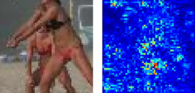
Figure 2. Volleyball.
Top 5 predictions: [‘bikini’, ‘pole’, ‘miniskirt’, ‘volleyball’, ‘swimming trunks’]
An excellent example where the saliency map focuses on the dark body of the black widow:
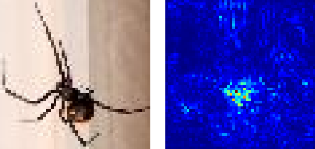
Figure 3. Black widow.
Top 5 predictions: [‘black widow’, ‘cockroach’, ‘tarantula’, ‘scorpion’, ‘fly’]
This zoom in of the wooden spoons do resemble frying pans.
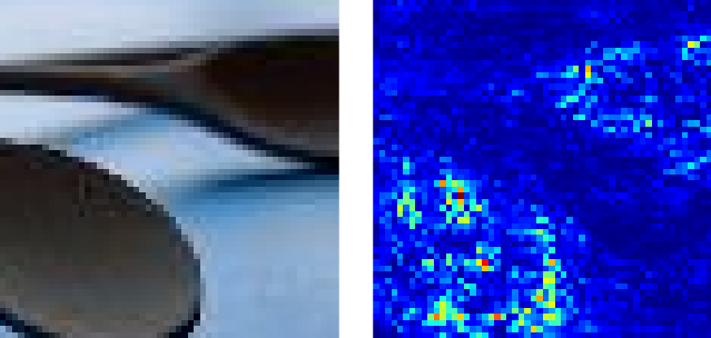
Figure 4. Wooden spoon.
Top 5 predictions: [‘frying pan’, ‘drumstick’, ‘nail’, ‘wooden spoon’, ‘reel’]
Examples like the one below are amazing. All five predictions are reasonable. And the saliency map is focused in on the claws: a defining feature of scorpions and lobsters.
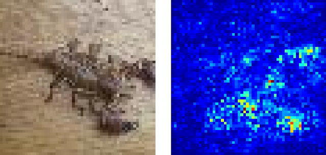
Figure 5. Scorpion.
Top 5 predictions: [‘scorpion’, ‘tailed frog’, ‘American lobster’, ‘cockroach’, ‘spiny lobster’]
Below is one more nice example where all five predictions are somewhat reasonable. And, honestly, I never would have figured out what this was. An open question is: Why is there such a bright spot of saliency at the middle top?
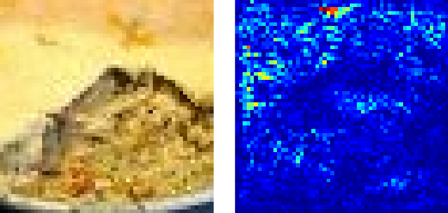
Figure 6. Potpie.
Top 5 predictions: [‘potpie’, ‘plate’, ‘mashed potato’, ‘guacamole’, ‘meat loaf’]
Kernel Visualization
It is interesting to view the Gabor-like filters in the early layers of the convnet. If these filters have more noise than structure, this can be a clue that your network is not well trained.
The receptive field is only 5x5 after the first two 3x3 layers. Even with 5x5 images, you can note the vertical, horizontal, diagonal, and spot-like patterns that are learned (Figure 7).
The receptive field after the 4th convolution is 11x11 and there is more fine-grained structure (Figure 8).
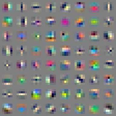
Figure 7. Visualization of 64 filters after 2nd 3x3 convolution. See Gist for notebook.
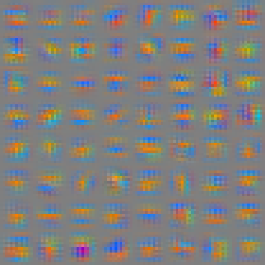
Figure 8. Visualization of 64 filters after 4th 3x3 convolution. See Gist for notebook.
Conclusion
The amazing achievements of convnets are well-publicized. By building and tuning your own convnet, you better understand their capabilities, and their shortcomings. With inexpensive cloud compute resources, and free software like Python and TensorFlow, this technology is accessible to almost anyone.
As always, I hope you’ve found this post useful. All the code is available in my GitHub repository. Please comment with any questions or suggestions for improvement.